
GET TO KNOW THE STEPS OF MAPBIOMAS METHODOLOGY
Below we detail the MapBiomas Venezuela methodology step by step. For each class and cross-cutting them covered in the map, there are specific characteristics that can be consulted in detail in the ATBD (Algorithm Theoretical Basis Document) and its annexes.

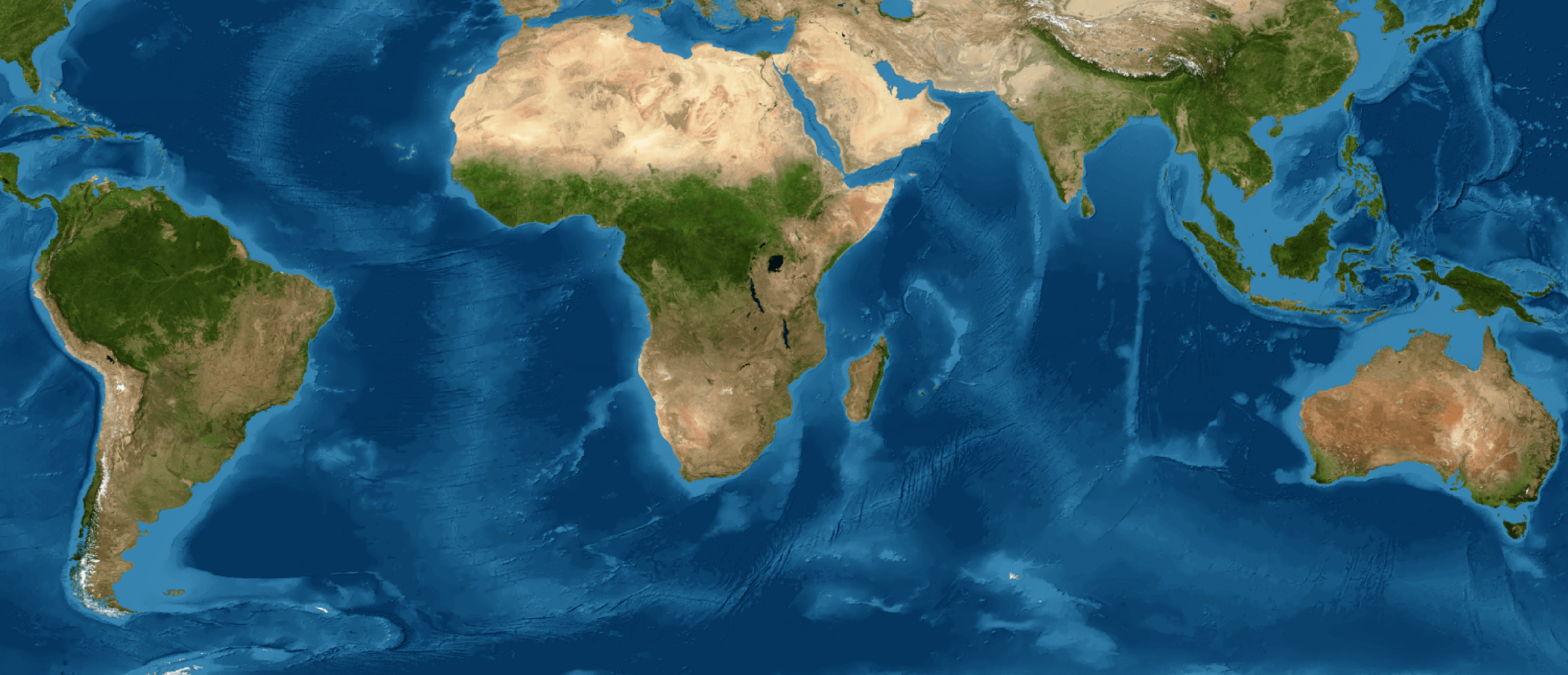
It all starts with Landsat satellite imagery, with a spatial resolution of 30 meters, available for free on the Google Earth Engine platform, from which a time series of annual mosaics is generated starting from 1985. Each of these mosaics summarizes information from the different Landsat images available for that year and is made up of tens of millions of pixels. These pixels constitute the MapBiomas methodology’s working units.
To produce each mosaic, cloud-free pixels are selected from the images available for the selected period to ensure the highest possible quality in the final image. Next, for each pixel, metrics are extracted that explain its behavior in that year and that provide the necessary information for its subsequent classification. This is done for each of the 7 spectral bands of the Landsat satellite, as well as with spectral fractions and indices calculated from them. For example, for the visible blue band the mosaic records the median value of the values of that band in the different images available for the period, as well as its maximum and minimum value and the amplitude of the variation. In the end, a given year's mosaic image includes up to 141 bands of information for each pixel.

For each year of the collection, a mosaic is generated that covers the entire country and represents the behavior of each pixel through the different metrics or information bands generated when constructing the mosaic. This set of mosaics is saved as a data collection (ASSET) within the Google Earth Engine platform and then used: 1) as a source of parameters for the image classification algorithm (see next step) and 2) to derive the RGB composition, which allows the display of the background image on the MapBiomas platform. This composition is also used for collecting training samples for the classification as well as samples for assessing accuracy through visual interpretation.
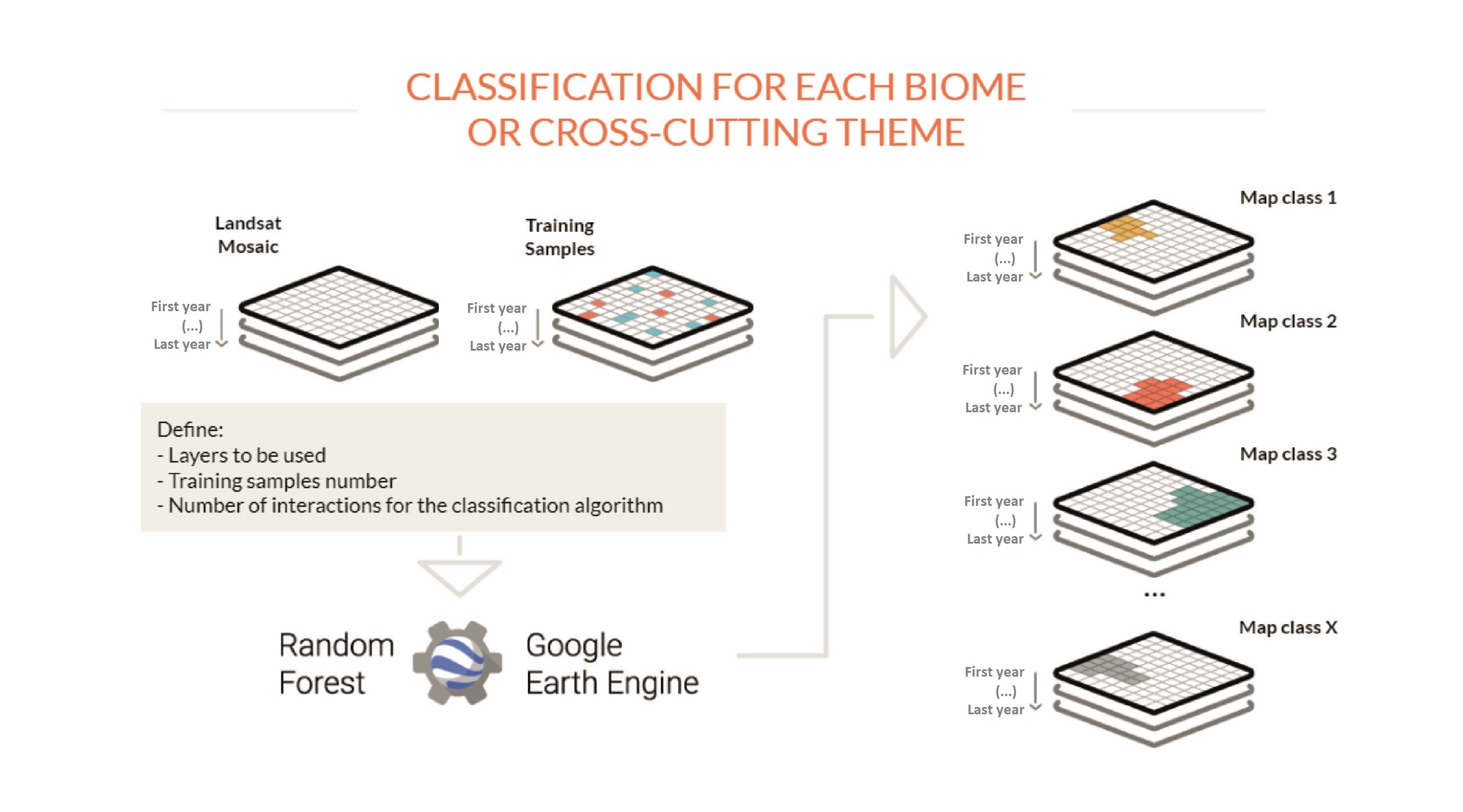
From the mosaics, the teams for each region and each cross-cutting theme produce a map of each type of land cover and use (Forest formation, Agriculture, Pasture, Urban use, Water body, etc.). To do so, MapBiomas analysts use an automatic classifier called “random forest”, which runs on Google Earth Engine (GEE). This system is based on machine learning: for each class to be classified, the machines are “trained” with samples of the targets to be classified. These samples can be obtained from reference maps, from the generation of stable class maps from previous MapBiomas collections, or from direct collection by visual interpretation of Landsat images by analysts. The classification is carried out for each of the years of the series, and can be saved as a single map per class, where each pixel has a number of layers corresponding to the number of years of the historical series analyzed.
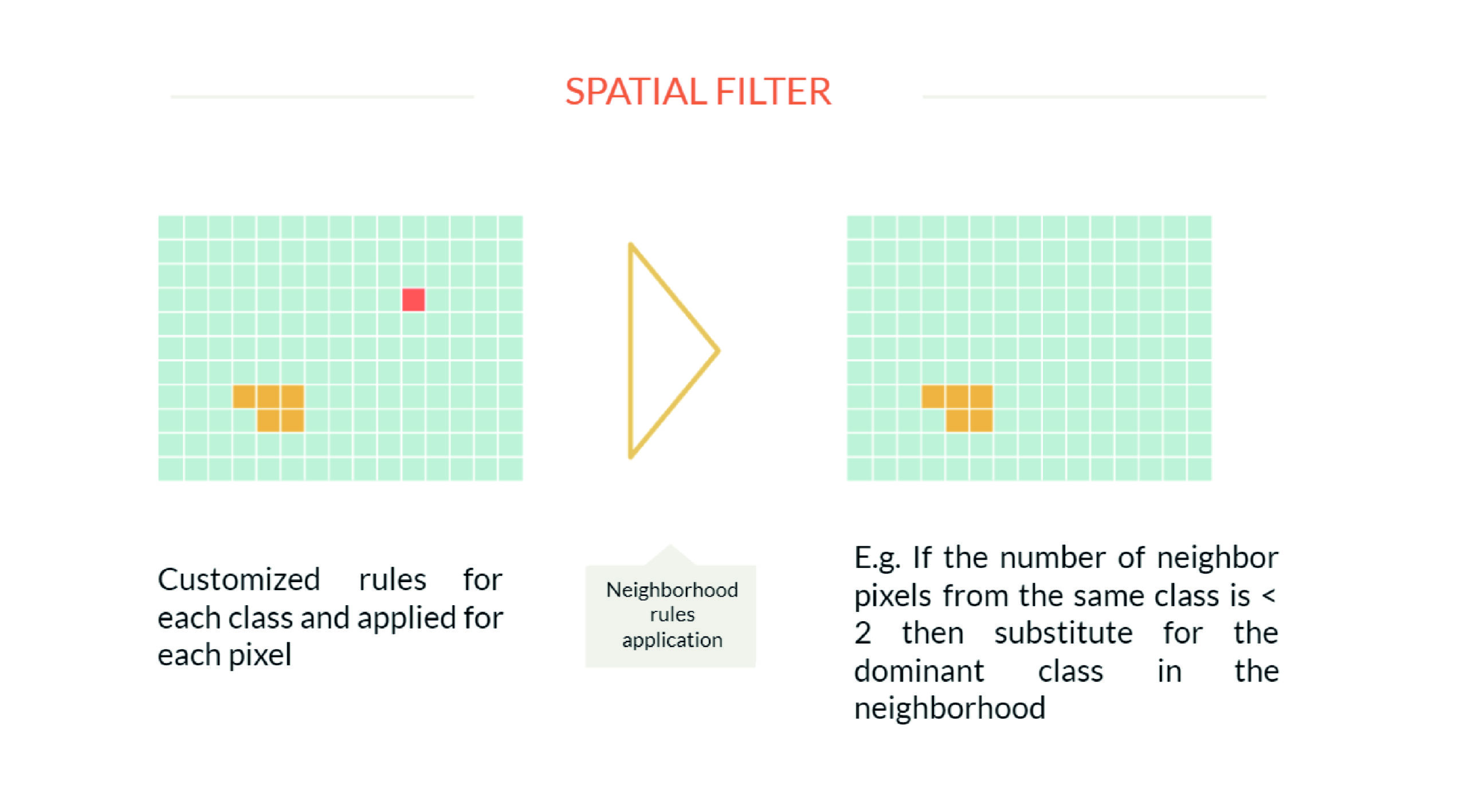
Once the initial classification has been generated, a spatial filter is applied, which aims to increase the spatial consistency of the data by eliminating isolated or border pixels. To do so, for each region and/or thematic class, neighborhood rules are defined that can lead to a change in the pixel classification. For example, a pixel that has fewer than two of nine neighboring pixels in the same class will be reclassified to the predominant class in the neighborhood. Each pixel in each year is subjected to spatial filtering.
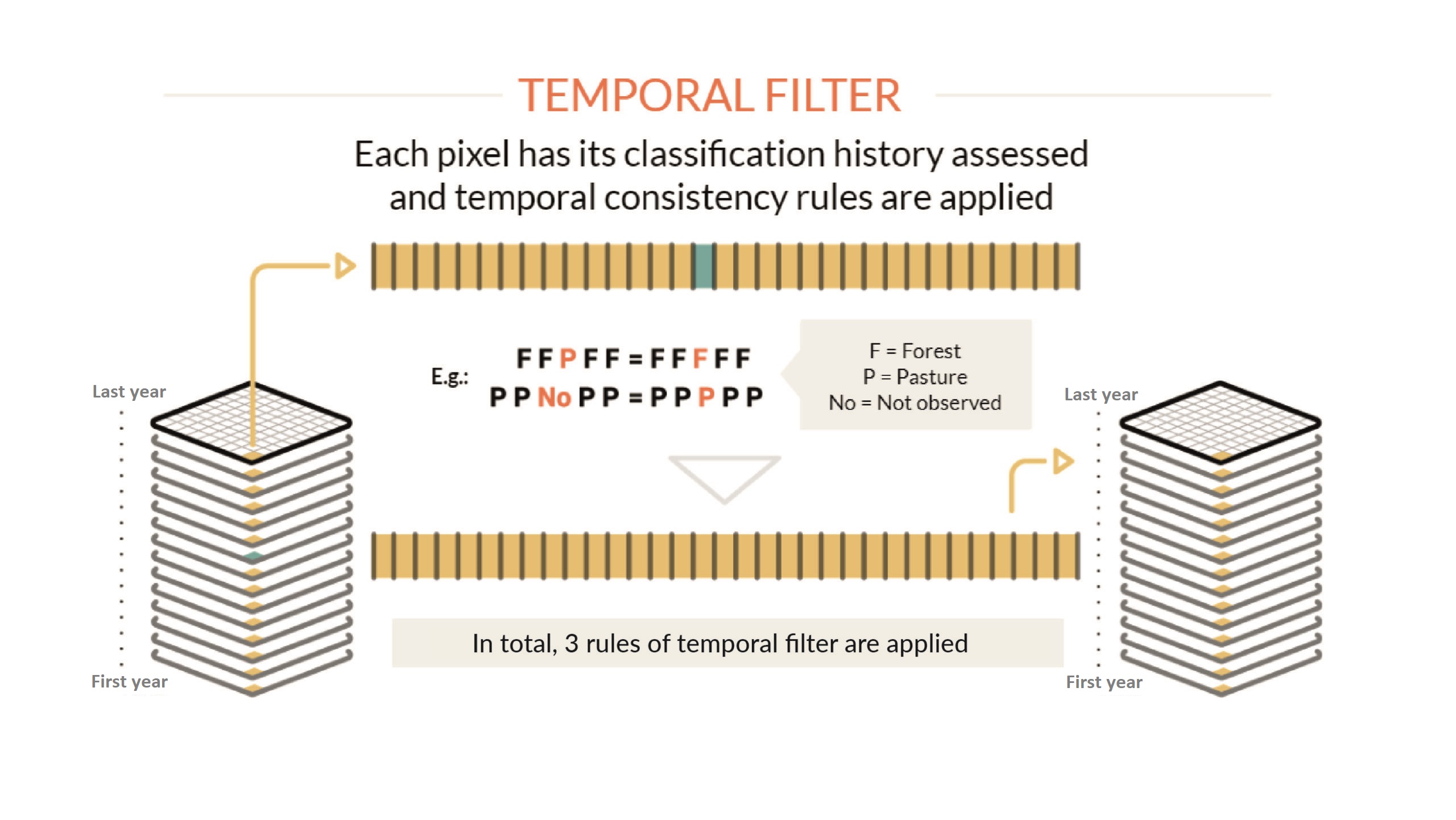
In addition to the spatial correction, the process can include the application of temporal filters that allow reducing temporal inconsistencies in the historical series of maps, especially those associated with “impossible” or “not permitted” changes in land cover and land use. (for example, the change in three consecutive years of the series of Natural forest > Non-forest > Natural forest). These filters also reduce failures due to excessive cloud cover or missing data in some years of the series. Each theme, or region can have specific temporal filter rules.
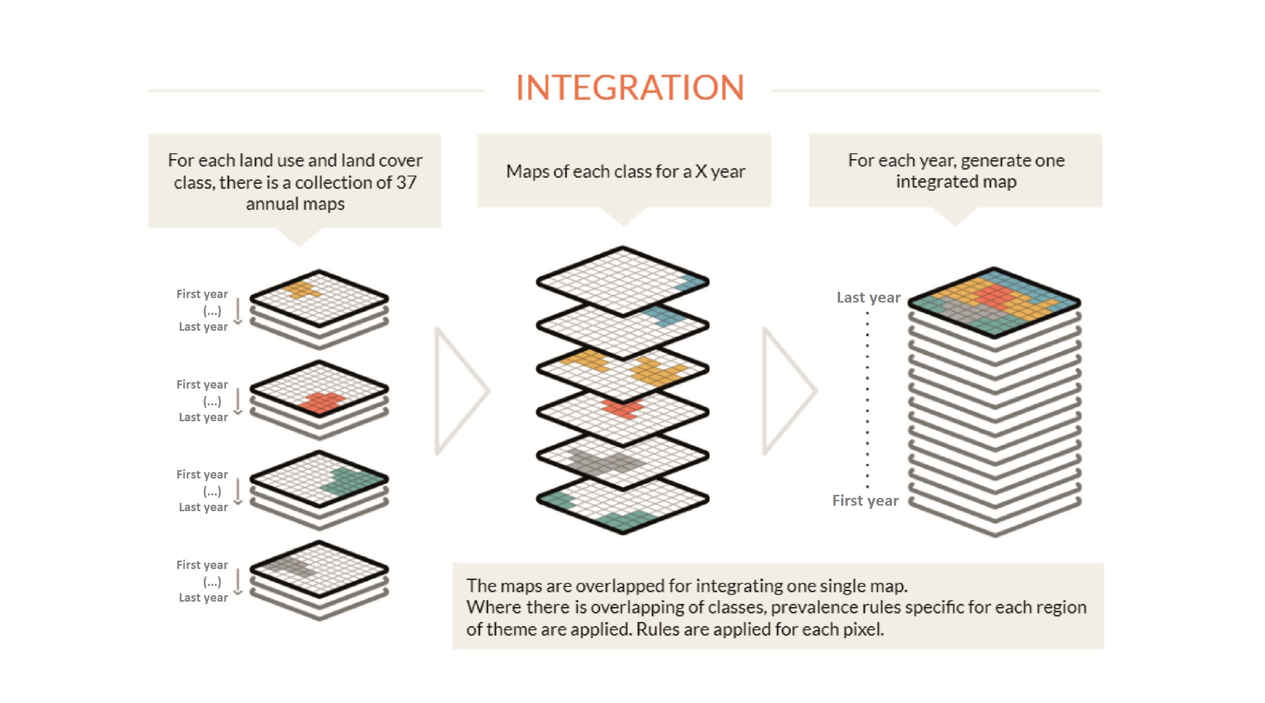
Once all the filters have been processed, the maps of each region and cross-cutting theme are integrated into a single map that represents the land use and land cover of the entire territory for each year. For this integration process, prevalence rules are applied; therefore, if the same pixel was classified in two maps of different classes, it is possible to define which class it belongs to in the final map. Rules of prevalence may vary depending on the peculiarities of themes or regions. The integration is performed for each year of the time series (i.e., an integrated map is generated for each year) and the result is usually saved as a single ASSET with the number of annual maps of the analyzed period (e.g., 40 maps for a period of 40 years). The integrated map goes through one more spatial filter step to clean up any edges and isolated pixels that are a result of the integration process.
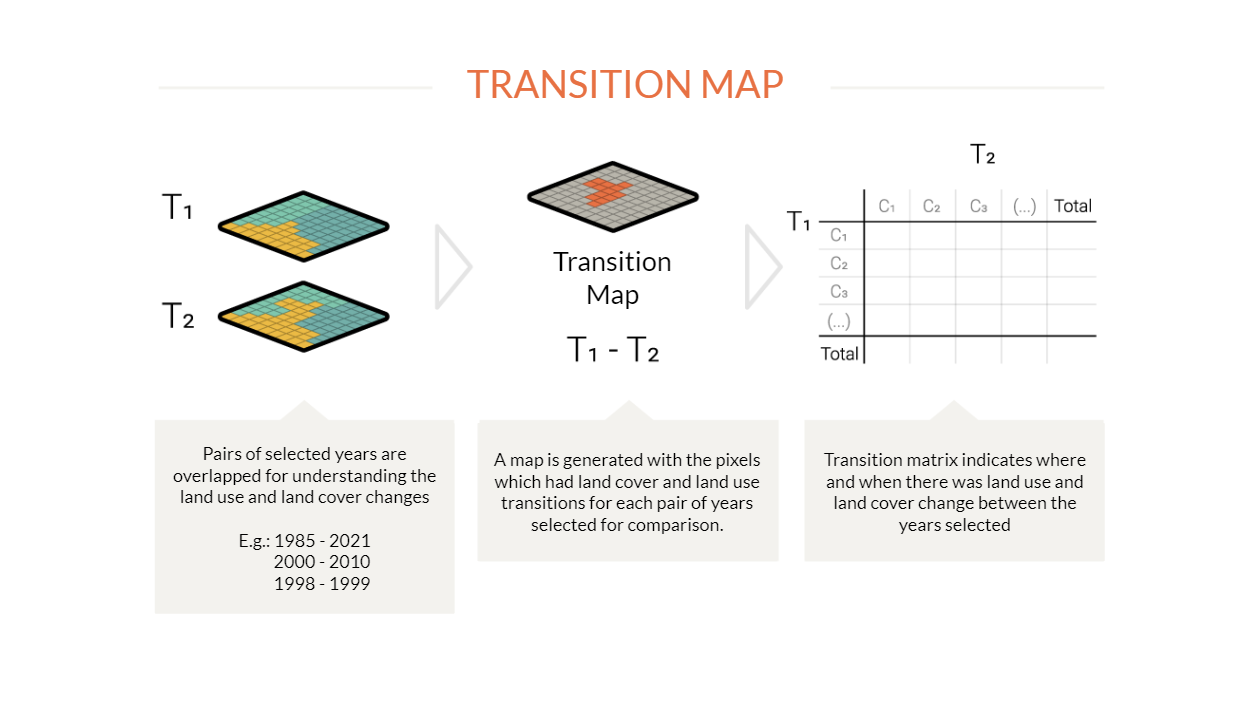
Finally, to understand changes in land cover and land use over time, maps with class transitions between different pairs of selected years are produced. Thus, it is possible to visualize the dynamism of the territory, and answer questions such as how much of the forest has been converted to pasture from one year to the next, as well as similar questions for other changes in the landscape. Transition maps are produced on a pixel-by-pixel basis and, once completed, are also subjected to a spatial filter to remove stray or edge transition pixels. From these maps, transition matrices are built for each state, municipality, type of protected area, indigenous territories and other territorial units available on the MapBiomas Venezuela platform.